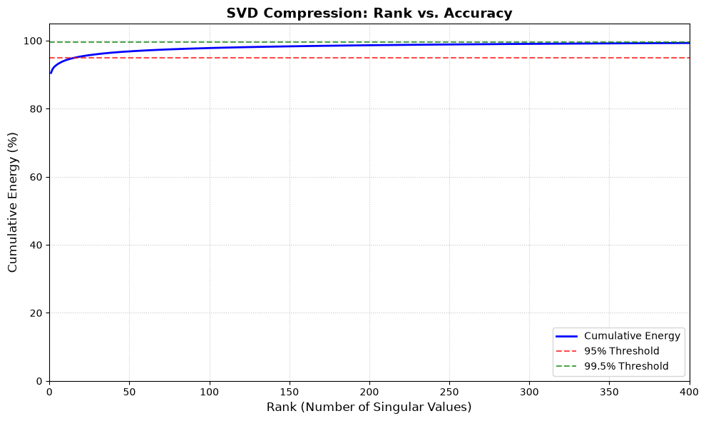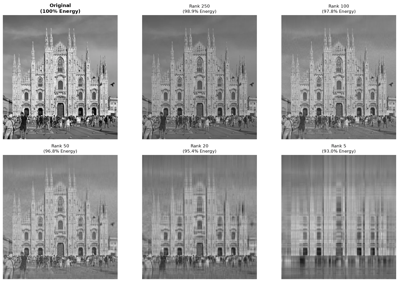
Singular Value Decomposition (SVD) is a fundamental algorithm in numerical linear algebra. In this post, I will show how to factorize a matrix and use low-rank approximation to compress a high-resolution image, using Python.
The Mathematics of SVD
Every real matrix $A$ of dimensions $m \times n$ can be factored into three matrix:
$$A = U \Sigma V^T$$
Where:
- $U$ is an $m \times m$ orthogonal matrix of left singular vectors.
- $\Sigma$ is an $m \times n$ diagonal matrix containing the singular values ($\sigma_i$) in descending order.
- $V^T$ is an $n \times n$ orthogonal matrix of right singular vectors.
By keeping only the largest $k$ singular values (where $k < \text{rank}(A)$), we can form a truncated approximation $A_k$ that captures the maximum possible “energy” (or variance) of original matrix:
$$A_k = U_k \Sigma_k V_k^T$$
The retained energy percentage is calculated by summing the squared singular values:
$$\text{Energy} = \frac{\sum_{i=1}^k \sigma_i^2}{\sum_{i=1}^n \sigma_i^2} \times 100$$
Factorizing a Matrix
First, let’s set up the environment and generate a $10 \times 10$ random matrix.
import numpy as np
import matplotlib.pyplot as plt
from PIL import Image

np.set_printoptions(precision=3, suppress=True)
rng = np.random.default_rng(seed=42)

mat = rng.uniform(0, 100, size=(10, 10))
print(mat)
[[77.396 43.888 85.86  69.737  9.418 97.562 76.114 78.606 12.811 45.039]
 [37.08  92.676 64.387 82.276 44.341 22.724 55.458  6.382 82.763 63.166]
 [75.809 35.453 97.07  89.312 77.838 19.464 46.672  4.38  15.429 68.305]
 [74.476 96.751 32.583 37.046 46.956 18.947 12.992 47.57  22.691 66.981]
 [43.715 83.268 70.027 31.237 83.226 80.476 38.748 28.833 68.25  13.975]
 [19.991  0.736 78.692 66.485 70.517 78.073 45.892 56.874 13.98  11.453]
 [66.84  47.11  56.524 76.5   63.472 55.358 55.921 30.395  3.082 43.672]
 [21.458 40.853 85.34  23.394  5.83  28.138 29.359 66.192 55.703 78.39 ]
 [66.431 40.639 81.402 16.697  2.271  9.005 72.236 46.188 16.127 50.104]
 [15.231 69.632 44.616 38.102 30.151 63.028 36.181  8.765 11.801 96.19 ]]
Now I define the functions I need to compute the SVD matrices $U$, $\Sigma$, and $V$, approximate the matrix, and calculate the cumulative energy.
def factorize(mat):
    """Decomposes a matrix into U, Sigma, and V."""
    U, sval, Vh = np.linalg.svd(mat, full_matrices=False)
    Sigma = np.diag(sval)
    V = Vh.T
    return U, Sigma, V


def approx_matrix(U, Sigma, V, rank):
    """Approximates the original matrix using truncated U, Sigma, and V."""
    U_r = U[:, :rank]
    Sigma_r = Sigma[:rank, :rank]
    V_r = V[:, :rank]
    return U_r @ Sigma_r @ V_r.T


def cum_energy(Sigma):
    """Calculates individual energies and cumulative variance percentage."""
    s = np.diag(Sigma)
    e = s**2
    total = np.sum(e)
    cum_var = np.cumsum(e) / total * 100
    return e, cum_var


U, Sigma, V = factorize(mat)
e, cum = cum_energy(Sigma)

print("Energies:", e)
print("Cumulative %:", cum)
Energies: [251111.204  17722.405  13647.473  10046.728   6727.073   5782.75
   3406.186   2028.353    522.858     18.857]
Cumulative %: [ 80.74   86.438  90.826  94.056  96.219  98.078  99.174  99.826  99.994
 100.   ]
As we can see, the very first singular value alone captures over 80% of the matrix’s variance!
SVD Image Compression
An image is just a 2D matrix of pixels. Let’s load the target image.
img = Image.open("cathedral.jpg").convert("L")
mat = np.array(img, dtype=float)

plt.imshow(mat, cmap="gray")
plt.title("Original")
plt.axis("off")
plt.show()
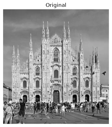
Attribution: Ludvig14, CC BY-SA 4.0, via Wikimedia Commons. Source
Now, I decompose the image matrix and find how many singular values (rank) are needed to retain 99.5% of the quality.
U, Sigma, V = factorize(mat)
e, cum = cum_energy(Sigma)

accuracy = 99.5
rank_accu = np.argmax(cum >= accuracy) + 1
print(f"Rank needed for {accuracy}% retained energy: {rank_accu}")
print(f"Actual energy retained at this rank: {round(cum[rank_accu - 1], 2)}%")
Rank needed for 99.5% retained energy: 510
Actual energy retained at this rank: 99.5%
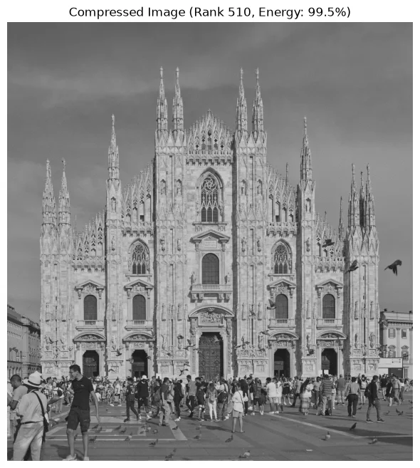
Using a rank of 510, I reconstruct the compressed image:
mat_accu = approx_matrix(U, Sigma, V, rank_accu)

plt.figure(figsize=(8, 8))
plt.imshow(mat_accu, cmap="gray")
plt.title(f"Compressed Image (Rank {rank_accu}, Energy: {accuracy}%)")
plt.axis("off")
plt.show()

Performance and Memory Optimization
Why do this? Because storing the truncated matrices $U$, $\Sigma$, and $V$ at a lower rank needs significantly fewer data points than storing the full original matrix.
# Compare Memory Size
m, n = mat.shape
r = rank_accu

original_elements = m * n
compressed_elements = r * (m + n + 1)
compression_ratio = (compressed_elements / original_elements) * 100

print(f"Image Dimensions:          {m}x{n}")
print(f"Original Storage Elements: {original_elements:,}")
print(f"SVD Storage Elements:      {compressed_elements:,}")
print(f"Compression Ratio:         {compression_ratio:.2f}%")
print(f"Total Memory Saved:        {100 - compression_ratio:.2f}%")
Image Dimensions:          4149x3840
Original Storage Elements: 15,932,160
SVD Storage Elements:      4,074,900
Compression Ratio:         25.58%
Total Memory Saved:        74.42%
We saved almost 75% of the memory while keeping close to the exact same image quality.
The Variance Curve
Plotting the cumulative energy clearly shows how fast it converges, within just a few hundred singular values.
ranks = np.arange(1, len(cum) + 1)
plt.figure(figsize=(10, 6))
plt.plot(ranks, cum, color="blue", linewidth=2, label="Cumulative Energy")
plt.axhline(y=95, color="red", linestyle="--", alpha=0.7, label="95% Threshold")
plt.axhline(y=99.5, color="green", linestyle="--", alpha=0.7, label="99.5% Threshold")
plt.title("SVD Compression: Rank vs. Accuracy", fontsize=14, fontweight="bold")
plt.xlabel("Rank (Number of Singular Values)", fontsize=12)
plt.ylabel("Cumulative Energy (%)", fontsize=12)
plt.xlim(0, 400)
plt.ylim(0, 105)
plt.grid(True, linestyle=":", alpha=0.7)
plt.legend(loc="lower right")
plt.tight_layout()
plt.show()