View the code on GitHub · Read the full honors report (PDF)
A full SVD gives the best rank-$k$ approximation of a matrix, but it is slow. For one dense 13,514 by 13,514 matrix it took about 640 seconds and 4 GB of memory on my computer. Randomized algorithms get close to the same answer in a few seconds. In this project I wrote three of them in Python (Gaussian rSVD, SRHT-rSVD and randQB_EI), tested them, and compared accuracy, runtime and memory on synthetic matrices and on kernel matrices from a boundary integral equation, with sizes up to 20,000 by 20,000.
The short version: the Gaussian and SRHT methods reach the same accuracy, and one power iteration brings either of them to within 1% of the exact SVD’s error. In theory SRHT should be faster, because it does far fewer operations. In my runs it was not. In my implementation it was 1.4 to 5 times slower than the Gaussian sketch and used 20 to 270 times more memory. A good part of this page is about why.
Background
The truncated SVD $A_k = U_k \Sigma_k V_k^T$ is the best rank-$k$ approximation of $A$ in the spectral and the Frobenius norm (Eckart-Young), and its Frobenius error is
$$\lVert A - A_k \rVert_F^2 = \sum_{i > k} \sigma_i^2$$
I use this as the baseline. Every error on this page is relative, $\lVert A - \hat A \rVert_F / \lVert A \rVert_F$, and I compare it with what the exact SVD gives at the same rank.
The randomized idea is to avoid decomposing $A$ directly. Multiply $A$ by a random matrix $\Omega$ with $l = k + p$ columns, where $p$ is a small oversampling margin (I use $p = 10$), and orthonormalize the result:
$$Y = A\Omega, \qquad Q = \mathrm{qr}(Y)$$
Now $Q$ spans roughly the same space as the top singular vectors of $A$, so $A \approx QQ^TA$. The SVD of the small matrix $Q^TA$ is cheap, and multiplying its left factor by $Q$ gives an approximate SVD of $A$. All three methods below follow this pattern. They differ in how they pick $\Omega$ and in when they stop.
The three algorithms
Gaussian rSVD. The entries of $\Omega$ are independent standard normal numbers. This is the method of Halko, Martinsson and Tropp. The dense product $A\Omega$ costs $O(mnl)$. If the singular values decay slowly, the basis can be improved with power iteration: use $(AA^T)^q A\Omega$ instead of $A\Omega$, so directions with large singular values are amplified. I run a QR factorization after every multiplication. Without it, all columns drift toward the top singular vector and the smaller directions are lost in rounding error.
SRHT-rSVD. Here $\Omega^T$ is a subsampled randomized Hadamard transform, $\Omega^T = \sqrt{N/l} \cdot R \cdot H \cdot D$. The matrix $D$ flips the sign of each coordinate at random, $H$ is the normalized Walsh-Hadamard matrix, and $R$ keeps $l$ randomly chosen rows. The transform needs a power-of-two size $N$, so the input is zero-padded from $n$ up to the next power of two. With the fast Walsh-Hadamard transform the sketch costs $O(mN \log N)$ instead of $O(mnl)$. The original method has no power iteration. I added it in the simplest way: sketch once with the SRHT, then run the same QR-based iteration as in the Gaussian version. I do not claim this is new. It is useful as a check, because with enough iterations both methods have to converge to the same answer.
randQB_EI. This method, by Yu, Gu and Li, does not take a rank. It takes a tolerance $\varepsilon$ and grows $Q$ and $B = Q^TA$ in blocks of $b = 10$ columns until $\lVert A - QB \rVert_F \le \varepsilon \lVert A \rVert_F$. The stopping test is cheap. Since $Q$ has orthonormal columns, $\lVert A - QQ^TA \rVert_F^2 = \lVert A \rVert_F^2 - \lVert B \rVert_F^2$, so the code only subtracts the squared norm of each new block from a running total.
Because randQB_EI has no rank input, I run it at several tolerances, record the rank where it stopped, and compare with the other two at that rank. This is not a perfectly like-for-like comparison, and I keep it in mind when reading the results.
All three accept dense NumPy arrays and SciPy sparse matrices.
Test matrices
The synthetic matrices are 2,000 by 2,000. Each is built as $U \Sigma V^T$ with random orthogonal $U$ and $V$ and chosen singular values: $\sigma_j = e^{-0.1 j}$ (exponential decay), $\sigma_j = 1/j$ (polynomial decay), and values near 1 with 5% noise (flat). The flat one is a control. Nothing should compress it, so a method that does well on it has a bug.
The main matrix is a discretized Laplace kernel,
$$K_{ij} = \frac{1}{4\pi \lVert x_i - y_j \rVert}$$
where the points $x_i$ lie on one unit sphere and the points $y_j$ on another unit sphere, with the two centers 2.1 apart. This is the potential of a point charge, the kind of block that appears when a boundary integral equation is discretized. The spheres never touch, so the kernel is smooth over the whole matrix and a short expansion approximates it well. This is the same reason fast multipole and hierarchical matrix methods work. I chose the separation of 2.1 so the singular values fall fast but not trivially: at $n = 13{,}514$ the exact SVD already reaches 1.4% error at rank 20.
I picked $n = 13{,}514$ on purpose. It is the size of the SuiteSparse matrix poisson3Da, which I had looked at first (more on that below). For the size comparison I also built a matrix with $n = 20{,}000$.
A full SVD is too slow to repeat at these sizes, so the reference for the kernel matrix comes from the top 250 singular values computed with scipy.sparse.linalg.svds, together with $\lVert A \rVert_F$ computed directly from the entries. The optimal error at rank $k$ needs only the top $k$ singular values and $\lVert A \rVert_F$, so this gives exact optimal errors for every rank up to 200.
How I measured
Each run records wall time, peak memory, and the relative Frobenius and spectral errors. Memory comes from tracemalloc, so it counts Python-level allocations including NumPy buffers, not the whole process. The errors are computed from the factors, without ever forming $A - U \Sigma V^T$. The Frobenius error uses $\lVert A \rVert_F^2 - 2\langle A, U \Sigma V^T \rangle + \lVert \Sigma \rVert_F^2$, and the spectral error takes the top singular value of the residual through an implicit operator. This matters for large or sparse matrices, where the dense residual would not fit in memory. Most settings were run with 12 random seeds, and the numbers below are means over those runs. The comparison with the exact SVD uses fewer seeds, because each full SVD takes so long. The ranks are 5, 10, 20, 50, 100 and 200, with $p = 10$.
Accuracy
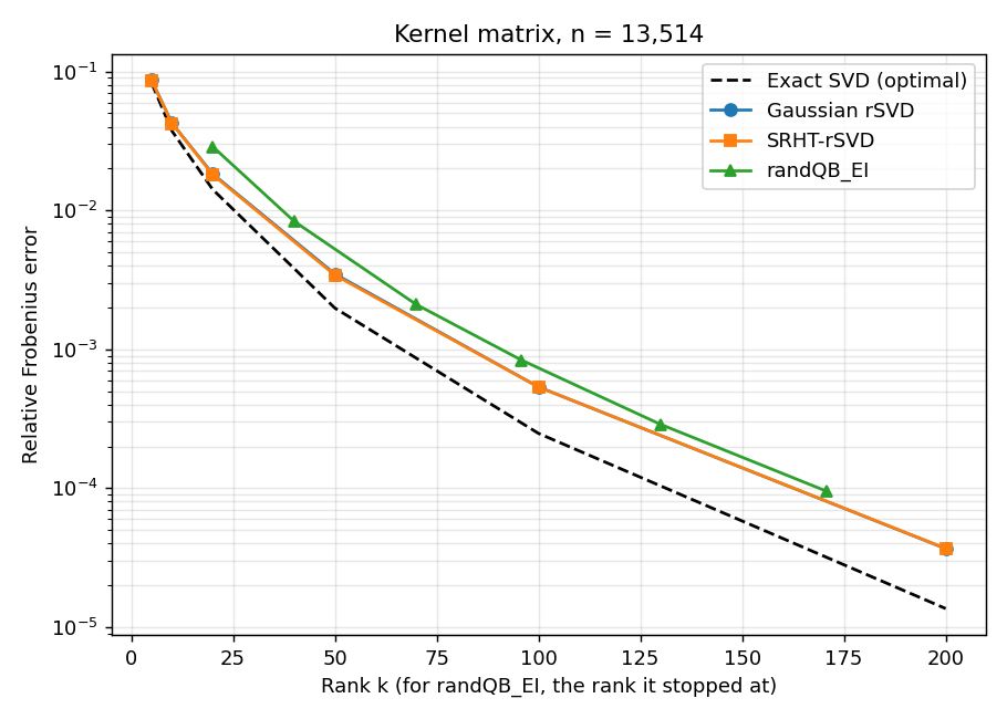
The plot at the top of this page shows the relative Frobenius error against rank for the $n = 13{,}514$ matrix. Gaussian and SRHT are almost one curve. At $k = 50$ the mean errors are 3.49e-3 and 3.42e-3, and the exact SVD gives 1.98e-3. At $k = 200$ they are 3.67e-5 and 3.68e-5 against 1.36e-5. Without power iteration, both stay within a factor of about 3 of the best possible error, and the factor grows slowly with rank: 1.05 at $k = 5$, 1.8 at $k = 50$, 2.7 at $k = 200$. The spectral error is the harder measure and shows the same pattern with a wider gap, about 4 times the optimum at $k = 200$. Both sketches use the same number of columns, which is probably why they agree so closely.
randQB_EI met its tolerance every time. I ran it with $\varepsilon$ from 0.05 down to 0.0001, 12 seeds each, and all 72 runs converged with a final error below $\varepsilon$.
| tolerance $\varepsilon$ | rank reached | relative error | runtime (s) |
|---|---|---|---|
| 0.05 | 20 | 0.0288 | 0.79 |
| 0.01 | 40 | 0.00835 | 1.30 |
| 0.003 | 70 | 0.00210 | 2.09 |
| 0.001 | 96 | 0.000836 | 2.80 |
| 0.0003 | 130 | 0.000288 | 3.73 |
| 0.0001 | 171 | 0.0000948 | 4.86 |
At the one rank where I ran both ($k = 20$), randQB_EI has an error of 0.0288 and Gaussian has 0.0183. It has no spare columns, and I think this is the reason. Its error stays between 2 and 3.3 times the optimum across all six tolerances. The extra cost buys the convenience of not having to guess the rank.
Power iteration
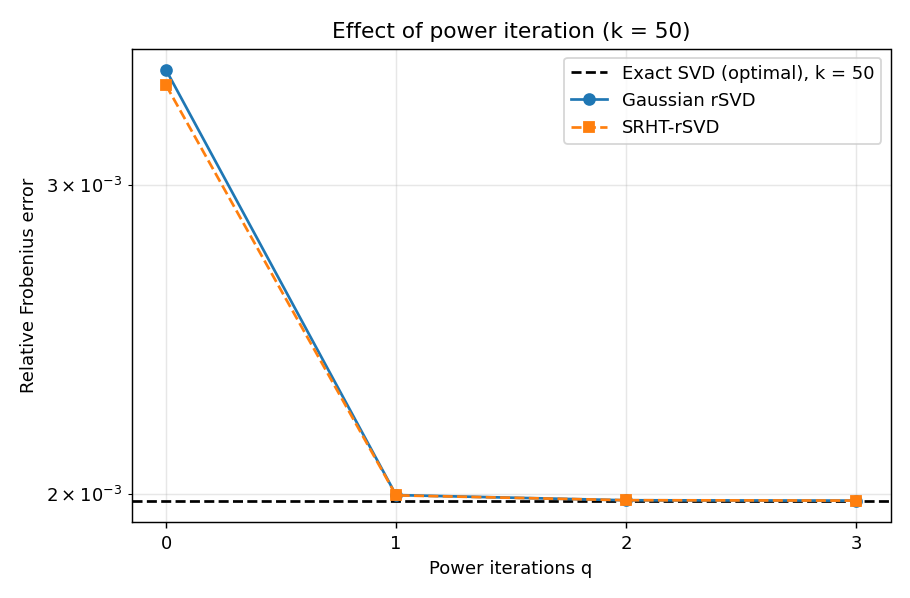
For the kernel matrix, one step is almost enough. At $k = 50$ the Gaussian error goes from 3.49e-3 at $q = 0$ to 2.00e-3 at $q = 1$, which is 0.8% above the exact SVD’s 1.98e-3. Steps 2 and 3 give 1.983e-3 and 1.982e-3, so they add nothing that I can see. They do cost time: 0.72, 1.45, 2.12 and 2.80 seconds for $q = 0$ to 3, about 0.7 seconds per step.
This is a fast-decaying spectrum, and it is the reason a single step is enough. On the slowly decaying polynomial matrix ($n = 2{,}000$, $k = 50$) the picture is different. The errors are 0.157, 0.1108, 0.1089 and 0.1085 for $q = 0$ to 3, against an optimum of 0.1083. One step leaves the error 2.3% above the optimum and three steps get within 0.2%.
The SRHT version with power iteration gives 1.982e-3 at $q = 3$ on the kernel matrix, the same as Gaussian to four digits. Since I added this part myself, I checked it in two ways: this agreement, and a test that compares it with gaussian_rsvd at $q = 3$.
Cost, and where SRHT loses
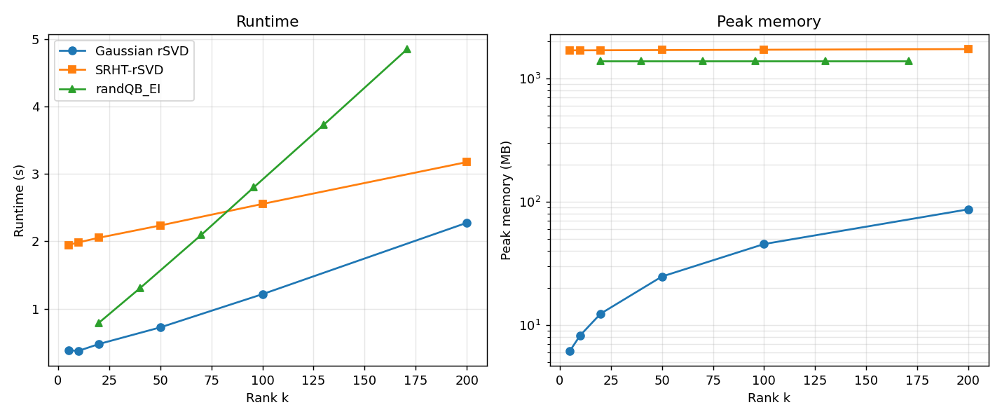
Gaussian takes 0.38 seconds at $k = 5$ and 2.3 seconds at $k = 200$, using between 6 and 87 MB. SRHT takes 1.9 to 3.2 seconds and about 1.7 GB, almost independent of $k$. There are two separate reasons.
The first is memory. The Hadamard transform is dense, even when the input is sparse. It works on a zero-padded array of $16{,}384 \times 13{,}514$ doubles, which is about 1.7 GB, and that size does not depend on the rank.
The second is speed per operation. I timed the sketch step alone at $l = 210$. Gaussian is one matrix product, $A\Omega$, with 76.7 GFLOP of work that finished in 0.90 seconds, about 85 GFLOP/s. By the count $2mN\log_2 N$, the SRHT needs 6.2 GFLOP, which is 12 times less, but it took 1.89 seconds, about 3.3 GFLOP/s. So SRHT did a twelfth of the work in twice the time, and its throughput was about 26 times lower. The Gaussian product runs inside a tuned BLAS library. My transform is a plain loop compiled with Numba. I also noticed that SRHT replaces only the first of the two large products in the algorithm. The second one, $Q^TA$, is dense in both methods, so even a perfect transform would save at most about half of the work.
The transform rewrite
My first version of the Walsh-Hadamard transform was much worse than these numbers. It rebuilt the whole array with np.concatenate at each of the 14 butterfly levels, and it transposed a C-contiguous array before reshaping, which silently forces a full copy every call. The rewrite does the butterfly in place along axis 0 on a single buffer and compiles it with Numba.
| matrix size | old time | old peak memory | new time | new peak memory |
|---|---|---|---|---|
| n = 2,000 | 0.206 s | 164 MB | 0.023 s | 39 MB |
| n = 13,514 | 15.0 s | 8,857 MB | 1.92 s | 1,817 MB |
Before timing, the script checks that the two versions give the same sketch (to $10^{-10}$ on the first 64 rows), and the new transform is tested against the explicit Hadamard matrix for sizes 1 to 64. I keep the old function in the repository (fwht_prefix) only for this comparison. After the rewrite the gap to Gaussian is much smaller. So part of the slowdown was a bug in my code, and the rest did not go away.
For larger inputs the sketch can be computed in batches of rows, which bounds the size of the padded array. At $n = 20{,}000$ the padded size is 32,768, and a single dense array would take about 5 GB. With batches of 1,000 rows it is about 260 MB, and the measured peak for SRHT stayed between 254 and 286 MB.
Does the size matter?
I repeated the whole sweep at $n = 20{,}000$, which is 48% larger.
| rank $k$ | error, n = 13,514 | error, n = 20,000 | ratio |
|---|---|---|---|
| 5 | 0.0868 | 0.0856 | 0.99 |
| 10 | 0.0425 | 0.0418 | 0.98 |
| 20 | 0.0183 | 0.0180 | 0.98 |
| 50 | 0.00349 | 0.00342 | 0.98 |
| 100 | 0.000535 | 0.000546 | 1.02 |
| 200 | 0.0000367 | 0.0000384 | 1.05 |
The two error curves lie on top of each other, so the rank needed for a given accuracy did not change with the size. That fits the explanation: the decay comes from the geometry, meaning how far apart the spheres are, and not from how many points I sample on them. The randQB_EI ranks also barely moved (about 96 and 98 for $\varepsilon = 0.001$). Two sizes are enough to see this trend, but not enough to claim a scaling law.
Compared with the exact SVD
Here every method and the full SVD were timed in one process, on the same matrix, so the ratios can be compared. This was not the case in my first attempt. There each notebook timed its own full SVD, and for the same 2,000 by 2,000 matrix one recorded 3.46 seconds and another 1.59 seconds. That made speedups from different notebooks impossible to compare.
| method, n = 13,514 | runtime | faster than full SVD | peak memory |
|---|---|---|---|
| full SVD | 637 s | 1x | 4,181 MB |
| Gaussian, $k = 50$ | 0.71 s | 900x | 25 MB |
| Gaussian, $k = 200$ | 2.17 s | 293x | 87 MB |
| SRHT, $k = 50$ | 2.37 s | 270x | 1,702 MB |
| SRHT, $k = 200$ | 3.24 s | 197x | 1,733 MB |
| randQB_EI, $\varepsilon = 0.001$ (rank 90) | 2.64 s | 242x | 1,393 MB |
The randomized rows are means over 3 seeds.
All the methods are far faster than the full SVD. On memory the picture is different: the SRHT peak is only 2.4 times below the full SVD, while Gaussian is 170 times below it at $k = 50$ and 48 times below at $k = 200$. The randQB_EI peak is exactly one dense copy of $A$ (1,393 MB at $n = 13{,}514$, and 3,052 MB at $n = 20{,}000$). It comes from np.sum(A * A), which builds a temporary array of the same size as $A$ when it computes $\lVert A \rVert_F^2$.
A matrix that does not compress
Before the kernel matrix I tried real matrices from SuiteSparse. The first was pde900, a 900 by 900 sparse matrix from a discretized PDE. It barely compresses. Even the exact SVD at rank 400 leaves 46% error, and at rank 800 out of 900 there is still 7%. Gaussian rSVD at rank 200 leaves 81% error against 70% for the optimum. randQB_EI shows the same thing: a tolerance of 0.2 needed rank 790.
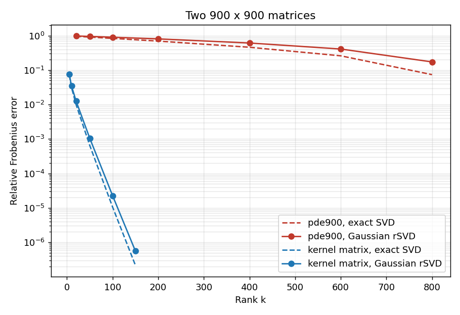
The kernel matrix of the same size behaves completely differently. Its exact error is 1.0% at rank 20 and about $10^{-5}$ at rank 100, and randQB_EI reaches a tolerance of 0.001 at rank 62. SuiteSparse also publishes the singular values of poisson3Da (13,514 by 13,514), and they decay slowly as well. This is why I moved to kernel matrices. A sparse matrix that comes from discretizing a differential operator couples only nearby points, and its singular values do not fall away quickly. An integral operator with a smooth kernel gives a dense matrix with fast decay. I kept the pde900 result in the repository as a negative result.
The synthetic matrices act as controls in the same way. On the exponential matrix, Gaussian gets 0.0105 at $k = 50$ against an optimum of 0.0067. On the flat matrix it gets 0.987 against 0.984, which means nothing was compressed, and randQB_EI never converged within its rank limit of 300. This is the correct behavior.
Limits
- I tested one kernel, the Laplace kernel between two well-separated spheres. Other kernels, or points that are close together, are known to be harder, and this is why hierarchical matrix methods exist.
- The matrices are constructed from a physical kernel. They are not measured data.
- There are only two sizes, so I did not test how anything scales.
- The SRHT result belongs to my implementation and my hardware. A multithreaded or vectorized transform might close the gap. I only showed that the gap survives one careful optimization pass.
- Peak memory is the
tracemallocpeak, which does not include memory allocated outside Python’s tracking.
Code and tests
The code is in the GitHub repository. The algorithms are in src/algorithms/, the experiment scripts in src/experiments/, and the CSV file behind every number on this page is committed next to its script. The figures here are drawn from those files. There are 58 tests. They check that sparse and dense input give the same factors, that the fast transform matches the explicit Hadamard matrix, and that the low-rank error functions agree with the dense formulas. One trap I hit: for a SciPy sparse matrix, A * A is a matrix product, not an elementwise square, so the Frobenius norm needs .multiply(). A test covers it. The package versions are pinned in requirements.txt.
References
- N. Halko, P.-G. Martinsson and J. A. Tropp, Finding structure with randomness: probabilistic algorithms for constructing approximate matrix decompositions, SIAM Review 53(2), 2011.
- C. Boutsidis and A. Gittens, Improved matrix algorithms via the subsampled randomized Hadamard transform, SIAM Journal on Matrix Analysis and Applications 34(3), 2013.
- J. A. Tropp, Improved analysis of the subsampled randomized Hadamard transform, Advances in Adaptive Data Analysis 3(1-2), 2011.
- W. Yu, Y. Gu and Y. Li, Efficient randomized algorithms for the fixed-precision low-rank matrix approximation, SIAM Journal on Matrix Analysis and Applications 39(3), 2018.
- L. Greengard and V. Rokhlin, A fast algorithm for particle simulations, Journal of Computational Physics 73(2), 1987.
- W. Hackbusch, A sparse matrix arithmetic based on H-matrices, Part I: Introduction to H-matrices, Computing 62, 1999.