This project has the ten problems I worked on in my MTH 5110 course, Numerical Methods for Differential Equations. I wrote every solver in Python from scratch as a short function, and each notebook states the problem, writes down the discretization and ends with a plot of either the convergence or the stability limit. All ten problems have an exact solution, so I could always compute the real error instead of trusting the output.
Boundary value problems
I started with a linear problem solved by central differences, where the tridiagonal system goes to solve_banded. The error dropped from 8.3e-3 at h = 1/10 to 1.3e-4 at h = 1/80, which is second order. For the nonlinear problem $y’’ = 1.5y^2$ I used Newton’s method with a tridiagonal Jacobian, and it converged in 4 iterations from the straight-line guess. Though it looks like it should have one answer, the problem has a second solution, and the starting guess $4 - 3x - c\sin(\pi x)$ with $c = 7$ reaches it. On top of that, I solved a third problem with hat functions (Rayleigh-Ritz), and on the same grids its error was almost the same as the finite difference one, so the finite element version had no real advantage there.
Elliptic problems
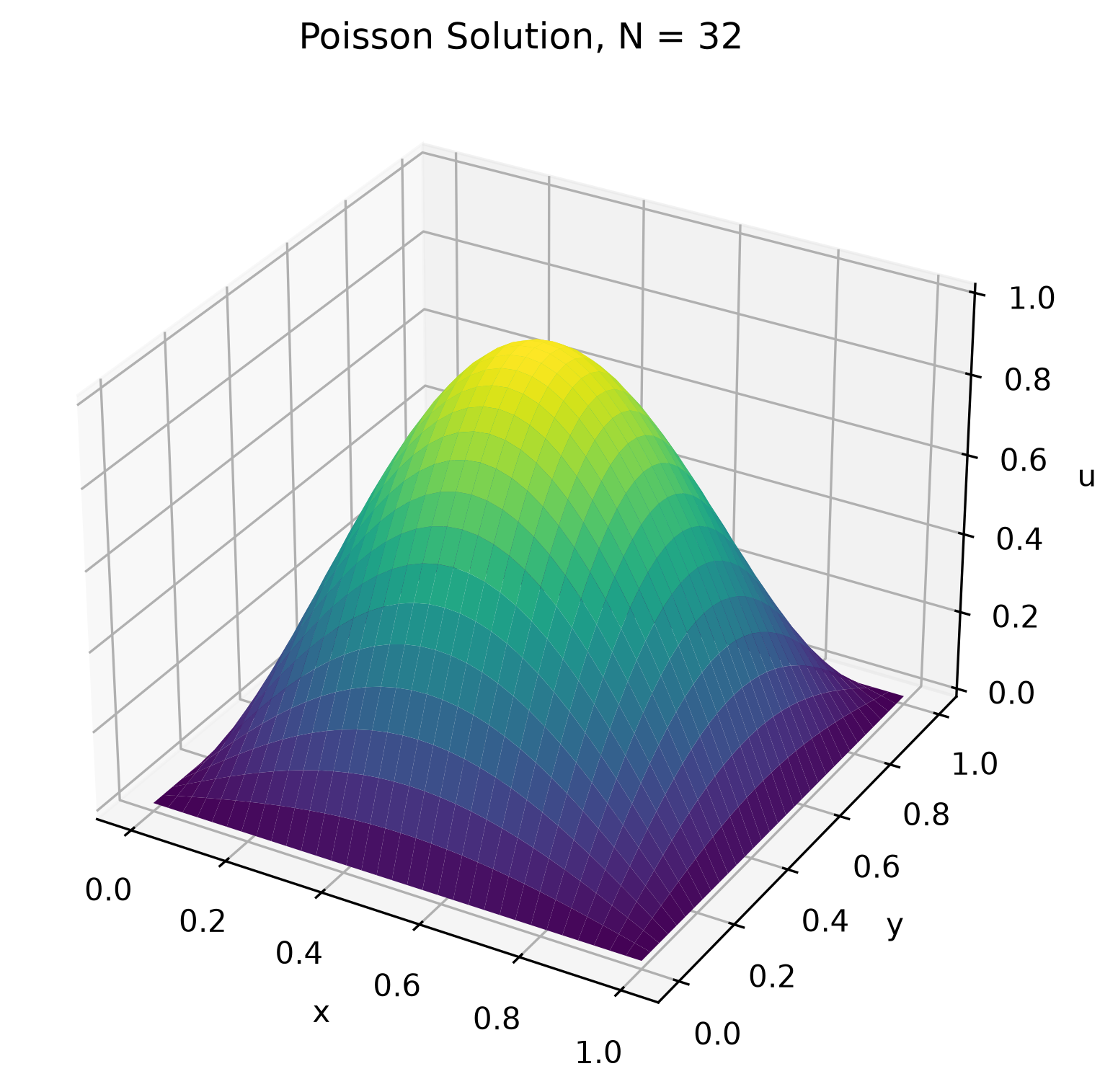
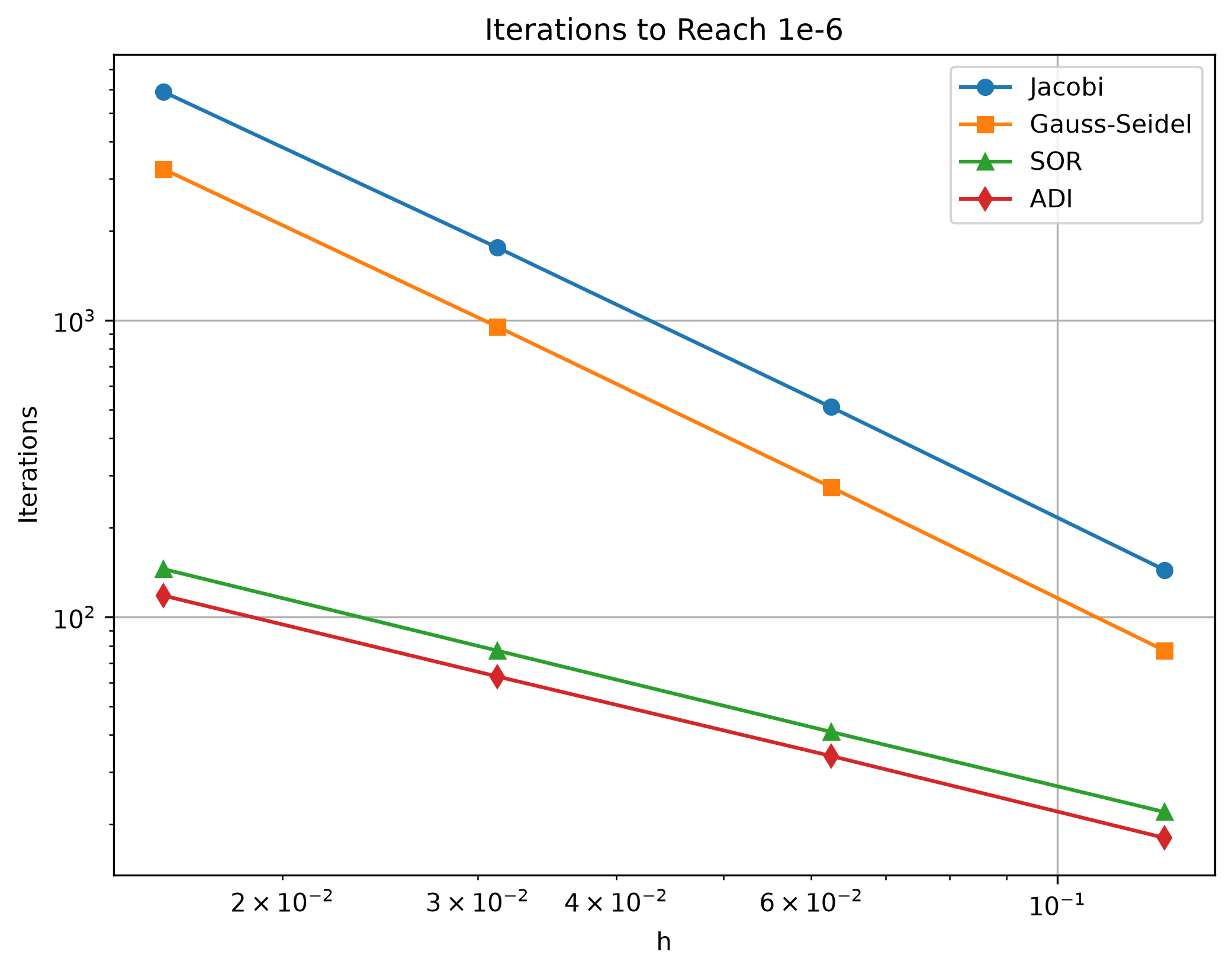
For the Poisson equation I built the five-point matrix with kron in scipy.sparse. At N = 64 it has 19,593 nonzeros, while a dense matrix would have 15.7 million entries, so the sparse form is the only reasonable choice. For Laplace I compared Jacobi, Gauss-Seidel and SOR, and at N = 64 SOR needed 140 iterations to reach 1e-6 against 2,857 for Gauss-Seidel and 5,138 for Jacobi. ADI needed 118 iterations on the Poisson problem where Jacobi needed 5,887, but SOR was still faster in runtime, because every ADI iteration does two sets of tridiagonal solves.
Time-dependent problems
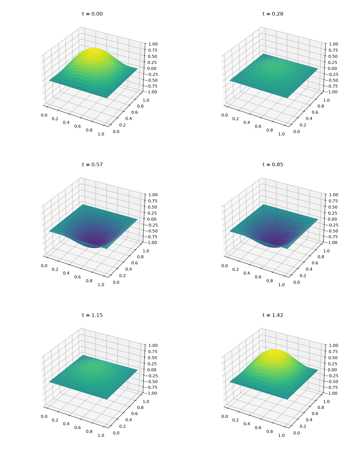
For the heat equation, the explicit scheme with r = 0.4 followed the exact solution with a max error of 1e-4, but with r = 0.6 and the hat initial condition it grew above 1e44 by t = 0.5. Crank-Nicolson stayed stable even at r = 5 and was second order in both $\Delta t$ and h. For the 1D wave equation, the error at Courant number $\sigma = 1$ was 5e-16, which is machine precision, and at $\sigma = 1.1$ rounding noise grew to 1e9 in 68 steps. The 2D version with $\Delta t = 0.9h/\sqrt{2}$ stayed bounded over a full period, and its error dropped by a factor of 4 each time I halved h.